Here you can find some of my data science
and machine learning projects on Python.
This portfolio is still under development,
feel free to visit again later.
Don't hesitate to reach out to me through any mean of communication
in the page footer.
About Me
From a fully non-technical background, I chose to undergo a career transformation and followed an intensive Data Science/AI bootcamp training at BeCode. Their self-learning-by-doing pedagogy was the perfect match to feed my eager to learn, gain and improve my skills in the vast and rapidly growing world of Data Science.
I'm passionate about data and its potential to drive insights and decision making in various industries and businesses. I'm enthusiastic about technologies and projects involving the implementation of Machine Learning Algorithm. I'm also a firm believer in continuous learning, specifically in a field with constant innovation. Don't hesitate to check on my resume which courses I'm following now.
After a successful internship, I'm actively looking for a Junior Data Scientist position as the next move in my career. If you feel we might have interests in common, feel free to contact me.
In this adaptation of the classic game, the player controls the snake with their index finger through the webcam. The goal is to eat as many Becode logos popping on the screen as possible to make the snake grow.
How It Works
When the game is launched, it triggers a while loop that maintains the interface open and constantly listens to the webcam signal - allowing it to show on the screen - and to the keyboard; if the "r" key is pressed, the game resets.
As soon as one hand is detected in the webcam (confidence of 0.8 with maximum one hand on the screen), a food object is instantiated at a random position in the playing area:
The tip of the player's index is what the head of the snake follows. Its position updates the coordinates of a "current_head" variable, passed to a "previous_head" variable, both of which help generate two lists: a list of previous index position coordinates and a list of distances between each of these points. The first one allows to draw the snake.
if self.points:
	for i, point in enumerate(self.points):
		if i != 0:
			cv2.line(img, self.points[i-1], self.points[i], (255, 0, 0), 15)
		cv2.circle(img, self.points[-1], radius=15, color=(255, 0, 0), thickness=cv2.FILLED)
The sum of all the lengths of the latter is compared with a "maximum_length" initial variable. When it exceeds this value, the oldest point and oldest segment (on index 0) are popped out of their respective lists.
if self.current_length > self.maximum_length:
	for i, length in enumerate(self.segments):
	    self.current_length -= length
	    self.segments.pop(i)
	    self.points.pop(i)
	    if self.current_length < self.maximum_length:
	        break
While the hand in the screen, the position of the index is compared with the rest of the snake body to check for collisions. To construct this function, the list of position points of the snake is converted into an array then passed into OpenCV methods to check for its distance. If between -1 and 1 pixel, the function returns True and the game stops.
if hands:
    landmark = hands[0]["lmList"]
    tip_index = landmark[8][0:2]
    if snake.check_for_collision(main_img):
        score.game_over(main_img)
    else:
        snake.update(main_img, tip_index)
Finally, the score.py file contains the functions updating the player's score everytime they eat a new cookie and displays the final scoreboard when the game is over.
Tools and technologies
Python | OOP | Computer Vision
NumPy
Math
Time
Random
OpenCV
CVZone
Extras
For demonstration purposes, the repository also contains:
A separated hand detection script
A separated face and features detection script
Future Developments
Setting up a highest Score Board
Game Over when hitting the border of screen as well
Setting options: starting lenght, colors, different choices of cookie design
Learning project consisting in plotting 3D representation of houses through the simple input of an address.
How It Works
After user inputs the desired address of the house, the program contacts the geopy API to fetch the proper GPS coordinates.
Those are then converted into the proper projection system (EPSG:31370 - Belgian Lambert 72 in this case).
These new coordinates can now be used to find the appropriate LIDAR data. To achieve this, they are compared with the bounding boxes coordinates inside the GeoTIFF files.
Once the altitudes matching the latitute and longitude projected coordinates are found, their value are added on an empty Numpy Array of dimension (200, 200).
It is finally used to render a 3D plot of the altitudes with Plotly.
def tiff_finder(x: float, y: float):
    paths = Path("./Data").glob("**/*.tif")
    loc = np.zeros((200, 200))
    for path in paths:
        with rasterio.open(path) as fd:
            if fd.bounds.left <= x <= fd.bounds.right:
                if fd.bounds.bottom <= y <= fd.bounds.top:
                    radius = 100
                    left, bottom, right, top = (
                        x - radius,
                        y - radius,
                        x + radius,
                        y + radius,
                    )
                    crop = fd.read(
                        1,
                        window=rasterio.windows.from_bounds(
                            left, bottom, right, top, fd.transform
                        ),
                    )
                    loc += crop
    fig = go.Figure(data=[go.Surface(z=loc)])
    fig.update_scenes(yaxis_autorange="reversed")
    fig.show()
Tools and Technologies
Python | OOP | GeoTIFF | Rasters | Data Visualization
NumPy
Geopy
Plotly
Pyproj
Rasterio
Future Developments
Tkinter or Kivy GUI
Data for the whole Belgium
Color map selection for 3D graphs
Toggle with/without Canopy Height Model
Visualizing only targetting specified house/building instead of area
API using a multiple linear regression model to predict prices of real-estate in Beligum based on a variety of criterias.
How It Works
First, approximately 18000 observations were scrapped from a popular real estate website. Price being identified as the target, the information from the website needed to be sorted in different features: property type, area, type of kitchen, the garden area if any, the number of facades, the general state, etc.
The whole set was saved into a pandas.DataFrame for more conveniance for the following operations.
Data preparation:
Remove duplicate observations and irrelevant ones
Feature selection to remove constant features, correlated ones to avoid multicollinearity (a correlation heatmap was used to highlight them)
Handling missing values: removing rows missing important data (no price, no area), replacing empty values with the median of all the other values of the column if continuous (ex.: surface), a 0 if meant to indicate absence (example: no garden), assuming some default values 1 for others (ex.: if no indication, it was always assumed there was at least one bathroom)
Feature Engineering: textual data transformed into numerical ordinal values (kitchen equipment, building state) or one-hot-encoded for nomial values (province, property type)
def mean_val(ref_col, target_col):
    ratios = target_col.divide(ref_col)
    mean = ratios.mean()
    default_values = ref_col.map(lambda x: x * mean, na_action="ignore")
    return target_col.fillna(default_values)

def none_to_default(value, default):
    if pd.isna(value):
        return default
    else:
        return value
Filter unwanted outliers: exceptional real estate (size, price, number of rooms) require a separate model due to their nature. The statistical Interquartile Range Method was used to remove them from the final dataset
feature engineering
One-Hot-Encoding for categorical data
Normalization: tests were conducted for two methods: MinMaxScaler and StandardScaler, the latter was showing slightly better results
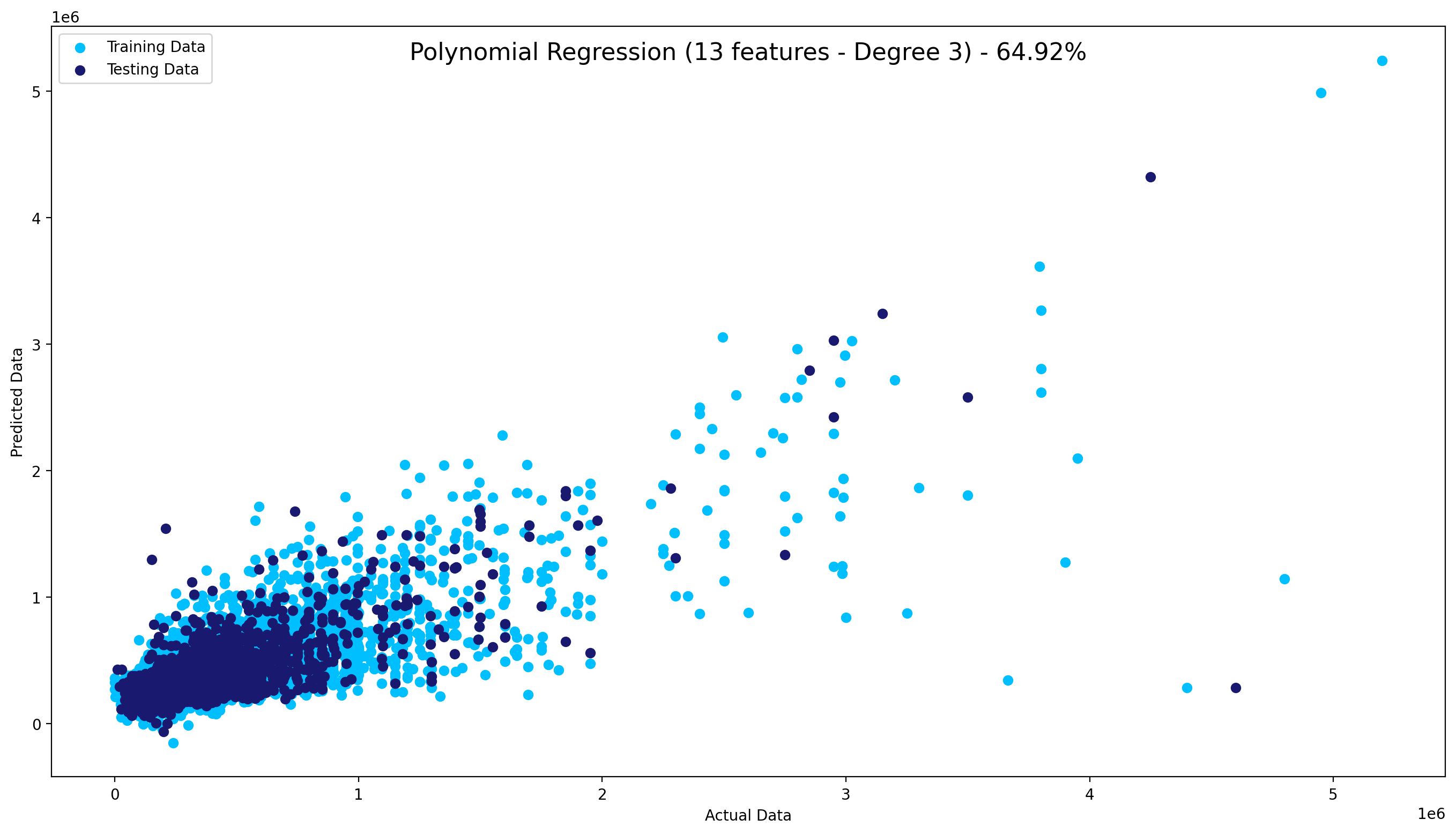
Model Selection:
The next step was to separate the data into a training and testing sets (0.8 / 0.2) using the scikit-learn dedicated function and testing different models; linear, multilinear and polynomial regressions.
The first one showed an R-squared of slightly under 55% while the polynomial model showed results above 60% with less features.
The multinear had close results and was chosen above Polynomial for performance concerns.
Deployment:
Use of Docker to containerise the trained model an Heroku for deployment as a micro-service app accessible through API.
Tests were conducted with Postman to check if the API was responsive and results as expected.
Please Refer to the API GitHub page for more information on how to format input.
Tools and Technologies
Python | Data Scraping | Data Cleaning | Feature Engineering | Visualization | Linear Regression | Multilinear Regression | Polynomial Regression | API | Containerisation
This project was developped to help UCL Neuroscience department to automate measures of delay in audio recording of patients suffering from stuttering.
These measures are used to evaluate patient's progresses and therapeutical protocoles.
It was realised in collaboration with Yasser Barona for the user interface.
How It Works
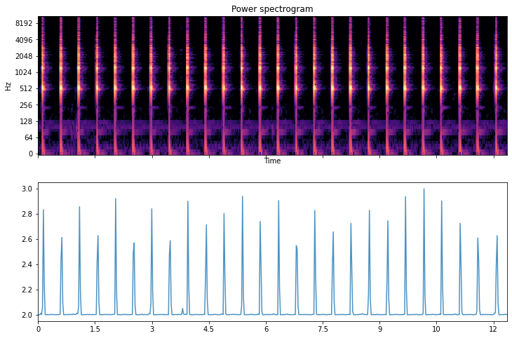
The audio files were structured as follow:
Each recorded session was 12 seconds long
The first 5 seconds were the metronome at 4 ticks per seconds
The patient was required to make a sound ("TA") after the 2 first "ticks" and try to follow the same rythm once the metronome stops
A virtual metronome sound file was used to create a list with the positions of reference of the ticks. A Librosa dedicated module using a peak-detection algorithm was used.
Due to recording conditions, Librosa failed at detecting all the peaks in patients' files. To bypass this issue and to avoid missing patients' "peaks" (i.e. when they were producing the required sound), a peak-detection algorithm was written from scratch using simple constrains;
as long as the sound signal was going up, the peak was not reached. Once it would go down, the latest high position was considered a peak if it was not too close from the previous one. After a few tweaking of the parameters of "distance" between sounds,
it managed to find all the peaks.
To make the comparison between the metronome reference file and the patients' recordings coordinates, the coordinates of the first one was aligned with the first 5 seconds peaks of the latter (i.e. where the metronome was audible in the patients' recording).
This step was primordial and constrained due to some recordings starting with up to 2 seconds of silence. Failing to do so would have given misleading results.
The following 7 seconds of peak of the patients' recording are then compared with the reference position of the metronome file. A RMSE (Root-Mean-Squared-Error) is then calculated to provide the results as a delay in seconds.
It quantifies the delta between the sounds pronounced by the patient and the time at which the metronome would have occured.
Deployment:
My colleague Yasser Barona implemented my code in a Streamlit interface to demonstrate the results to the Research Team of Université Catholique de Louvain.
Simplicity of use was the target; a simple form in which the user inputs 1 or a batch of sound files. Once the files submitted and the computations processed, the application outputs a csv with information such as peak-position, metronome position, patient position, RMSE for each peak, global RMSE.
Tools and Technologies
Python | Signal Processing | Peak Detection Algorithm
This Fake News Detection system was built in the context of deepening my understanding and practice of NLP Pipeline.
The word2vec-google-news-300 pre-trained model from Gensim library was used for word and sentence embeddings.
This pre-trained model was trained on approximately 100 billion words and contains around 300 million vectors.
How It Works
Using the Fake News Dataset from Kaggle, the first step was to prepare the data itself.
For more convenience, the two csv files (one for the fake news, the other for the real news) were concatenated in a
single Pandas DataFrame and only the necessary columns were kept: the content of the articles and their labels.
These were mapped in an additional column with numerical values; 0 for fake news, 1 for real news.
As our pretrained model requires a vector of a specific shape ((300,)), a function will transform the content of our articles using the
SpaCy Large English Pipeline. It contains a vocabulary of over half a million words and has strong NER (Name Entity Recognition) and POS (Part of Speech) abilities.
The function follows these steps:
Tokenize: each word of the text is isolated as a separate element of a list, becoming a single object denoted token
Filter out tokens that are either punctuation or a stop word as they would only add noise to our vectors
Lemmatize the tokens: the words are converted into their meaningful common forms (lemma) through vocabulary and morphological analysis (ex.: was -> be, better -> good)
Vectorize our tokens: through a semantic representation of our tokens (Word2Vec), the Gensim model will create a mathematical average (Sent2Vec) of the complete text for each article to be able to
depict the relashionships between sentences, and words inside our documents. This process is called Sentence Embedding
def preprocess_and_vectorize(text):
	doc = nlp(text)
	filtered_token = list()
	for token in doc:
		if token.is_punct or token.is_stop:
			continue
		filtered_token.append(token.lemma_)
	return wv.get_mean_vector(filtered_token)
After applying this function to each row of our DataFrame, we can train our Gradient Boosting Classifier model.
As usual, we first split the data in a train set and a test set then reshape it in a 2D vector to before fitting the model.
The Gradient Boosting Classifier is an Ensemble Method. Instead of using a single predictor, multiple predictors with poor accuracy
and their results are aggregated, usually allowing for a model with better accuracy. Boosting is a special type of Ensemble Learning technique
that, instead of fitting a predictor on the data at each iteration, actually itteratively fits a new predictor to the residual errors made by the previous predictor.
We can now make prediction on our test set and return a classification report as well as plot a confusion matrix.
This project was developped to give an insight on future Stock Trends and display the results in a WebApp.
Disclaimer
This project was thought as a coding/ML exercise. The predictions depicted by the model shouldn't be used as a financial
advise and should be considered cautiously; bevahiours of the market in the past are not proof nor signs of future behaviours.
I never aimed at giving any investments adices through this application and declines all responsability for the potential consequences
of any investment decisions made using this work.
How It Works
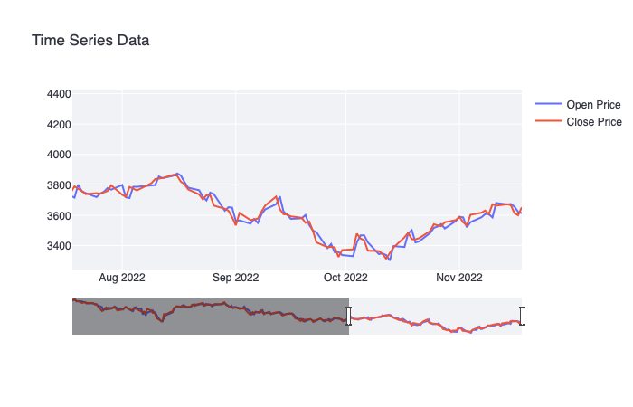
The user selects a ticker* in the selection box at the top making the WebApp sends a request to the Yahoo Fiance API to fetch
financial data from the starting date selected; the Opening Price, the Closing Price, The highest price for the day, the lowst
price for the day, the adjusted closing price and the daily volume.
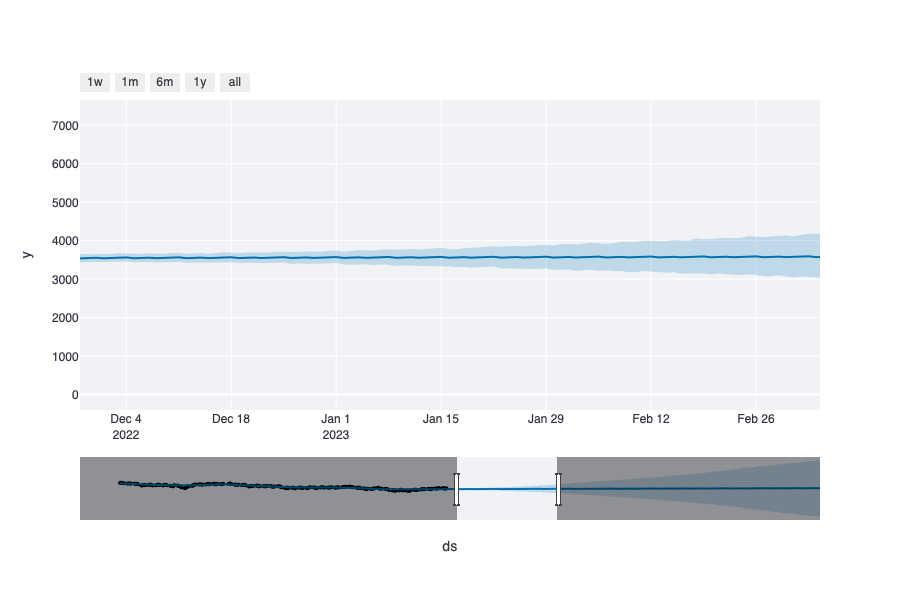
A slider is also made available for the user to decide how far the future predicition should be made; I set the default minimum value to 1 and its maximum to 10.
Any modification of these fields will instantly trigger the program to fetch new data and produce new predictions.
*Those starting with a ^ are general indices such as BEL20 or FTSE. Their real stock reference was used as a name; BEL20 as such is ^BFX
START = st.date_input("Starting date for historical data:")
TODAY = date.today().strftime("%Y-%m-%d")
n_years = st.slider("Years of prediction:", 1, 10)
period = n_years * 365


@st.cache # Streamlit cache to prevent loading the data everytime
def load_data(ticker):
    data = yf.download(ticker, START, TODAY)
    data.reset_index(inplace=True)
    return data
Plotly was used to enhance the user experience and offer an interactive visualization of selected ticker starting from
the selected date up to the last available data (typically, the previous day). In example above, a situation of the BEL20 Index since July 2022.
I used of a Prophet forecasting model to predict the Stock Trends. This open source library
is an ideal choice for time series predictions since it is based on an additive model - a non parametric regression method - that prevents
the data to become sparse when its space volume increases. This phenomenon is frequent in high-dimensional data leading to exponential
growth of its size.
The forecast is illustrated in a graph, again making use of plotly. In the following illustration, a prediction of BEL20 trend in the next few month.
Tools and Technologies
Python | Time Series | WebApp | Dashboard | Forecasting Model
This is bold and this is strong. This is italic and this is emphasized.
This is superscript text and this is subscript text.
This is underlined and this is code: for (;;) { ... }. Finally, this is a link.
Heading Level 2
Heading Level 3
Heading Level 4
Heading Level 5
Heading Level 6
Blockquote
Fringilla nisl. Donec accumsan interdum nisi, quis tincidunt felis sagittis eget tempus euismod. Vestibulum ante ipsum primis in faucibus vestibulum. Blandit adipiscing eu felis iaculis volutpat ac adipiscing accumsan faucibus. Vestibulum ante ipsum primis in faucibus lorem ipsum dolor sit amet nullam adipiscing eu felis.
Preformatted
i = 0;

while (!deck.isInOrder()) {
    print 'Iteration ' + i;
    deck.shuffle();
    i++;
}

print 'It took ' + i + ' iterations to sort the deck.';